Eğitim
How to Use Conditional Formatting with Checkboxes in Excel 365?
Let’s explore how to manage data using checkboxes in Excel 365 versions. In this article, we will demonstrate how to automatically highlight an entire row when a specific condition is met.
Adding Conditional Formatting with Checkboxes in a Table
In our dataset, we have three different groups labeled A, B, and C. Our goal is to apply a conditional formatting rule that highlights the entire row when all three groups are checked.
Step 1: Insert Checkboxes into the Table
- First, edit the table and select the data range where you want to apply the checkboxes.
- Go to the Insert menu and select Checkbox to add checkboxes to the selected range.
- When you click on a checkbox, it will return either TRUE (checked) or FALSE (unchecked).
Step 2: Apply Conditional Formatting
- Select the entire table where you want the row highlighting to appear.
- Click on Conditional Formatting in the Home tab and select New Rule.
- Choose Use a formula to determine which cells to format.
- Enter the following formula
=AND($F3=TRUE, $G3=TRUE, $H3=TRUE)
Here,$F3,$G3, and$H3represent the checkbox cells in the table. - Click Format, go to the Fill tab, and select a color to highlight the row.
- Press OK to apply the rule.
Step 3: Testing the Conditional Formatting
- When all three checkboxes in a row are checked, the entire row will be highlighted.
- If any of the checkboxes are unchecked, the row will return to its default formatting.
Conclusion
Thanks to the checkboxes introduced in Excel 365, performing such operations has become much easier. Conditional formatting with checkboxes is a great way to visually manage data, making it easier to track approvals or completed tasks.
See you in the next tutorial!